Decision Transformers

什么是离线强化学习？

深度强化学习 (RL) 是构建决策$Agents$的框架。这些$Agents$旨在通过反复试验与环境交互并接收奖励作为独特的反馈来学习最佳行为（策略）。

$Agents$的目标是最大化其累积奖励，称为回报。因为 RL 基于奖励假设：所有目标都可以描述为期望累积奖励的最大化。

深度强化学习$Agents$通过批量经验进行学习。问题是，他们如何收集数据？：

在线和离线设置中强化学习的比较，图片来自这篇文章

在线强化学习中，$Agents$直接收集数据：它通过与环境交互来收集一批经验。然后，它会立即（或通过一些重播缓冲区）使用此经验来从中学习（更新其策略）。

但这意味着你要么直接在现实世界中训练你的$Agents$，要么有一个模拟器。如果没有，则需要构建它，这可能非常复杂（如何在环境中反映现实世界的复杂现实？）、昂贵且不安全，因为如果模拟器有缺陷，如果它们提供竞争优势，$Agents$就利用它们。

另一方面，在离线强化学习中，$Agents$仅使用从其他$Agents$或人类演示中收集的数据。它不与环境相互作用。

过程如下：

1. 使用一个或多个策略和/或人工交互创建数据集。
2. 在此数据集上运行离线 RL 以学习策略

这种方法有一个缺点：反事实查询问题。如果我们的$Agents$人决定做一些我们没有数据的事情，我们该怎么办？例如，在十字路口右转，但我们没有这个轨迹。

已经有一些关于这个主题的解决方案，但如果你想了解更多关于离线强化学习的信息，你可以观看这个视频

引入 Decision Transformers

Decision Transformer 模型由 Chen L. 等人的“Decision Transformer：Reinforcement Learning via Sequence Modeling”介绍。它将强化学习抽象为条件序列建模问题。

主要思想是，我们不是使用 RL 方法训练策略，例如拟合值函数，它会告诉我们采取什么动作来最大化回报（累积奖励），我们使用序列建模算法（Transformer），给定期望的回报、过去的状态和动作将产生未来的动作以实现这一期望的回报。它是一个自回归模型，以期望回报、过去状态和动作为条件，以生成实现期望回报的未来动作。

这是强化学习范式的彻底转变，因为我们使用生成轨迹建模（对状态、动作和奖励序列的联合分布建模）来取代传统的 RL 算法。这意味着在 Decision Transformers 中，我们不会最大化回报，而是生成一系列未来的动作来实现预期的回报。

这个过程是这样的：

1. 我们将最后 K 个时间步输入到具有 3 个输入的Decision Transformer中：
   • Return-to-go
   • 状态
   • 动作
2. 如果状态是向量，则嵌入线性层；如果状态是帧，则嵌入 CNN 编码器， 对 Token 进行编码。
3. 输入由 GPT-2 模型处理，该模型通过自回归建模预测未来的行为。

Decision Transformers 架构。状态、动作和回报被送到模态特定的线性嵌入中，并添加了位置情景时间步长编码。Token 被送入 GPT 架构，该架构使用因果自注意掩码自回归地预测动作。图来自[1]。

在 🤗 Transformers 中使用Decision Transformer

Decision Transformer 模型现在作为 🤗 transformers 库的一部分提供。此外，我们还分享了 Gym 环境中连续控制任务的九个预训练模型。

“专家”Decision Transformer模型，在 Gym Walker2d 环境中使用离线强化学习学习。

安装包

pip install git+https://github.com/huggingface/transformers

加载模型

使用 Decision Transformer 相对容易，但由于它是一个自回归模型，因此必须小心谨慎，以便在每个时间步准备模型的输入。我们准备了一个Python 脚本和一个Colab 笔记本来演示如何使用该模型。

在 🤗 transformers 库中加载预训练的 Decision Transformer 很简单：

from transformers import DecisionTransformerModel

model_name = "edbeeching/decision-transformer-gym-hopper-expert"
model = DecisionTransformerModel.from_pretrained(model_name)

创造环境

我们为 Gym Hopper、Walker2D 和 Halfcheetah 提供预训练检查点。Atari 环境的检查点将很快可用。

import gym
env = gym.make("Hopper-v3")
state_dim = env.observation_space.shape[0] # state size
act_dim = env.action_space.shape[0] # action size

自回归预测函数

该模型执行自回归预测；也就是说，在当前时间步t做出的预测顺序地取决于先前时间步长的输出。这个功能很丰富，所以我们的目标是在评论中解释它。

# Function that gets an action from the model using autoregressive prediction
# with a window of the previous 20 timesteps.
def get_action(model, states, actions, rewards, returns_to_go, timesteps):
    # This implementation does not condition on past rewards

    states = states.reshape(1, -1, model.config.state_dim)
    actions = actions.reshape(1, -1, model.config.act_dim)
    returns_to_go = returns_to_go.reshape(1, -1, 1)
    timesteps = timesteps.reshape(1, -1)

    # The prediction is conditioned on up to 20 previous time-steps
    states = states[:, -model.config.max_length :]
    actions = actions[:, -model.config.max_length :]
    returns_to_go = returns_to_go[:, -model.config.max_length :]
    timesteps = timesteps[:, -model.config.max_length :]

    # pad all tokens to sequence length, this is required if we process batches
    padding = model.config.max_length - states.shape[1]
    attention_mask = torch.cat([torch.zeros(padding), torch.ones(states.shape[1])])
    attention_mask = attention_mask.to(dtype=torch.long).reshape(1, -1)
    states = torch.cat([torch.zeros((1, padding, state_dim)), states], dim=1).float()
    actions = torch.cat([torch.zeros((1, padding, act_dim)), actions], dim=1).float()
    returns_to_go = torch.cat([torch.zeros((1, padding, 1)), returns_to_go], dim=1).float()
    timesteps = torch.cat([torch.zeros((1, padding), dtype=torch.long), timesteps], dim=1)

    # perform the prediction
    state_preds, action_preds, return_preds = model(
            states=states,
            actions=actions,
            rewards=rewards,
            returns_to_go=returns_to_go,
            timesteps=timesteps,
            attention_mask=attention_mask,
            return_dict=False,)
    return action_preds[0, -1]

评估模型

为了评估模型，我们需要一些额外的信息；训练期间使用的状态的均值和标准差。幸运的是， Hugging Face Hub 上的每个模型卡都可以使用这些！

我们还需要模型的目标回报。这就是以回报为条件的离线强化学习的力量：我们可以使用目标回报来控制政策的表现。这在多人游戏设置中可能非常强大，我们希望调整对手机器人的性能，使其处于适合玩家的难度。作者在他们的论文中展示了一个很好的情节！

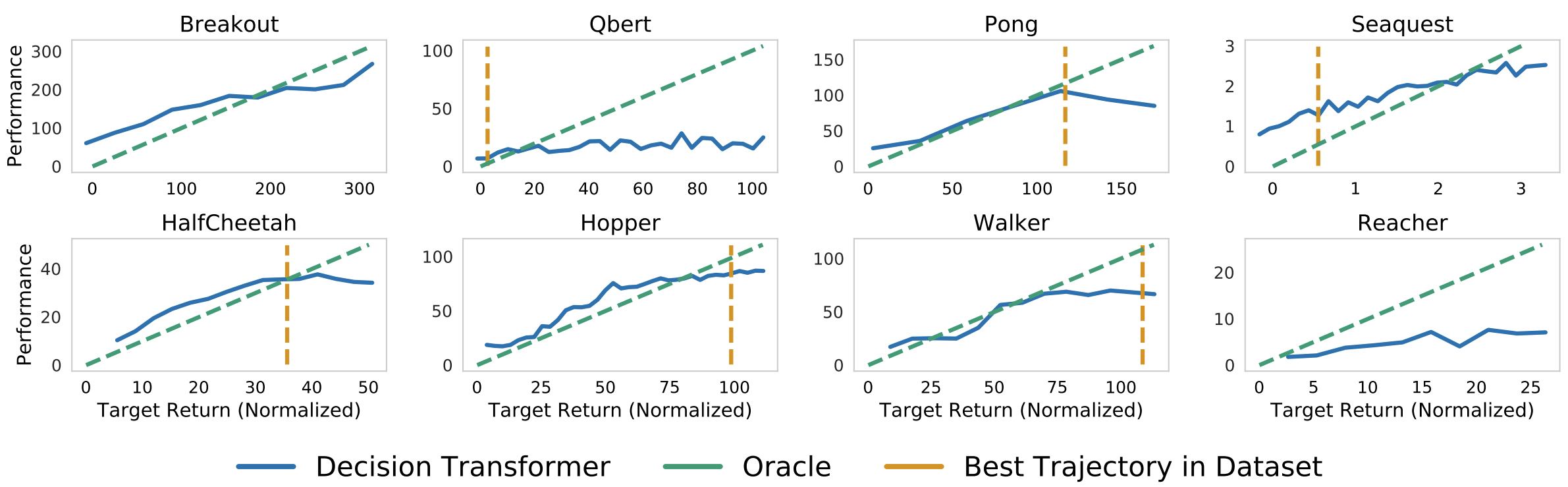在以指定目标（期望）回报为条件时，由 Decision Transformer 累积的采样（评估）回报。上：雅达利。底部：D4RL 中重放数据集。图来自[1]。

TARGET_RETURN = 3.6 # This was normalized during training
MAX_EPISODE_LENGTH = 1000

state_mean = np.array(
    [1.3490015,  -0.11208222, -0.5506444,  -0.13188992, -0.00378754,  2.6071432,
     0.02322114, -0.01626922, -0.06840388, -0.05183131,  0.04272673,])

state_std = np.array(
    [0.15980862, 0.0446214,  0.14307782, 0.17629202, 0.5912333,  0.5899924,
         1.5405099,  0.8152689,  2.0173461,  2.4107876,  5.8440027,])

state_mean = torch.from_numpy(state_mean)
state_std = torch.from_numpy(state_std)

state = env.reset()
target_return = torch.tensor(TARGET_RETURN).float().reshape(1, 1)
states = torch.from_numpy(state).reshape(1, state_dim).float()
actions = torch.zeros((0, act_dim)).float()
rewards = torch.zeros(0).float()
timesteps = torch.tensor(0).reshape(1, 1).long()

# take steps in the environment
for t in range(max_ep_len):
    # add zeros for actions as input for the current time-step
    actions = torch.cat([actions, torch.zeros((1, act_dim))], dim=0)
    rewards = torch.cat([rewards, torch.zeros(1)])

    # predicting the action to take
    action = get_action(model,
                        (states - state_mean) / state_std,
                        actions,
                        rewards,
                        target_return,
                        timesteps)
    actions[-1] = action
    action = action.detach().numpy()

    # interact with the environment based on this action
    state, reward, done, _ = env.step(action)

    cur_state = torch.from_numpy(state).reshape(1, state_dim)
    states = torch.cat([states, cur_state], dim=0)
    rewards[-1] = reward

    pred_return = target_return[0, -1] - (reward / scale)
    target_return = torch.cat([target_return, pred_return.reshape(1, 1)], dim=1)
    timesteps = torch.cat([timesteps, torch.ones((1, 1)).long() * (t + 1)], dim=1)

    if done:
        break

您会在我们的Colab notebook中找到更详细的示例，以及$Agents$视频的创建。

Training Decision Transformers

在这一部分中，我们将使用 🤗 Trainer 和自定义数据收集器从头开始训练Decision Transformers模型，使用 🤗 集线器上托管的离线 RL 数据集。您可以在这个 colab notebook中找到本教程的代码

我们将执行离线强化学习以在mujoco halfcheetah 环境中学习以下行为。

“专家”Decision Transformers 模型，在 Gym HalfCheetah 环境中使用离线强化学习学习。

加载数据集并构建自定义数据整理器

我们在hub上托管了许多离线 RL 数据集。今天，我们将使用 hub 上托管的 halfcheetah“专家”数据集进行训练。

首先，我们需要load_dataset从 🤗 数据集包中导入函数，并将数据集下载到我们的机器上。

from datasets import load_dataset
dataset = load_dataset("edbeeching/decision_transformer_gym_replay", "halfcheetah-expert-v2")

虽然集线器上的大多数数据集都可以开箱即用，但有时我们希望对数据集执行一些额外的处理或修改。在这种情况下我们希望匹配作者的实现，即我们需要：

• 通过减去平均值并除以标准差来归一化每个特征。
• 预先计算每个轨迹的折扣回报。
• 将奖励和回报乘以 1000 倍。
• 增加数据集采样分布，以便将专家代理轨迹的长度考虑在内。

为了执行此数据集预处理，我们将使用自定义 🤗 Data Collator 。

现在让我们开始使用用于离线强化学习的自定义数据整理器。

@dataclass
class DecisionTransformerGymDataCollator:
    return_tensors: str = "pt"
    max_len: int = 20 #subsets of the episode we use for training
    state_dim: int = 17  # size of state space
    act_dim: int = 6  # size of action space
    max_ep_len: int = 1000 # max episode length in the dataset
    scale: float = 1000.0  # normalization of rewards/returns
    state_mean: np.array = None  # to store state means
    state_std: np.array = None  # to store state stds
    p_sample: np.array = None  # a distribution to take account trajectory lengths
    n_traj: int = 0 # to store the number of trajectories in the dataset

    def __init__(self, dataset) -> None:
        self.act_dim = len(dataset[0]["actions"][0])
        self.state_dim = len(dataset[0]["observations"][0])
        self.dataset = dataset
        # calculate dataset stats for normalization of states
        states = []
        traj_lens = []
        for obs in dataset["observations"]:
            states.extend(obs)
            traj_lens.append(len(obs))
        self.n_traj = len(traj_lens)
        states = np.vstack(states)
        self.state_mean, self.state_std = np.mean(states, axis=0), np.std(states, axis=0) + 1e-6

        traj_lens = np.array(traj_lens)
        self.p_sample = traj_lens / sum(traj_lens)

    def _discount_cumsum(self, x, gamma):
        discount_cumsum = np.zeros_like(x)
        discount_cumsum[-1] = x[-1]
        for t in reversed(range(x.shape[0] - 1)):
            discount_cumsum[t] = x[t] + gamma * discount_cumsum[t + 1]
        return discount_cumsum

    def __call__(self, features):
        batch_size = len(features)
        # this is a bit of a hack to be able to sample of a non-uniform distribution
        batch_inds = np.random.choice(
            np.arange(self.n_traj),
            size=batch_size,
            replace=True,
            p=self.p_sample,  # reweights so we sample according to timesteps
        )
        # a batch of dataset features
        s, a, r, d, rtg, timesteps, mask = [], [], [], [], [], [], []

        for ind in batch_inds:
            # for feature in features:
            feature = self.dataset[int(ind)]
            si = random.randint(0, len(feature["rewards"]) - 1)

            # get sequences from dataset
            s.append(np.array(feature["observations"][si : si + self.max_len]).reshape(1, -1, self.state_dim))
            a.append(np.array(feature["actions"][si : si + self.max_len]).reshape(1, -1, self.act_dim))
            r.append(np.array(feature["rewards"][si : si + self.max_len]).reshape(1, -1, 1))

            d.append(np.array(feature["dones"][si : si + self.max_len]).reshape(1, -1))
            timesteps.append(np.arange(si, si + s[-1].shape[1]).reshape(1, -1))
            timesteps[-1][timesteps[-1] >= self.max_ep_len] = self.max_ep_len - 1  # padding cutoff
            rtg.append(
                self._discount_cumsum(np.array(feature["rewards"][si:]), gamma=1.0)[
                    : s[-1].shape[1]   # TODO check the +1 removed here
                ].reshape(1, -1, 1)
            )
            if rtg[-1].shape[1] < s[-1].shape[1]:
                print("if true")
                rtg[-1] = np.concatenate([rtg[-1], np.zeros((1, 1, 1))], axis=1)

            # padding and state + reward normalization
            tlen = s[-1].shape[1]
            s[-1] = np.concatenate([np.zeros((1, self.max_len - tlen, self.state_dim)), s[-1]], axis=1)
            s[-1] = (s[-1] - self.state_mean) / self.state_std
            a[-1] = np.concatenate(
                [np.ones((1, self.max_len - tlen, self.act_dim)) * -10.0, a[-1]],
                axis=1,
            )
            r[-1] = np.concatenate([np.zeros((1, self.max_len - tlen, 1)), r[-1]], axis=1)
            d[-1] = np.concatenate([np.ones((1, self.max_len - tlen)) * 2, d[-1]], axis=1)
            rtg[-1] = np.concatenate([np.zeros((1, self.max_len - tlen, 1)), rtg[-1]], axis=1) / self.scale
            timesteps[-1] = np.concatenate([np.zeros((1, self.max_len - tlen)), timesteps[-1]], axis=1)
            mask.append(np.concatenate([np.zeros((1, self.max_len - tlen)), np.ones((1, tlen))], axis=1))

        s = torch.from_numpy(np.concatenate(s, axis=0)).float()
        a = torch.from_numpy(np.concatenate(a, axis=0)).float()
        r = torch.from_numpy(np.concatenate(r, axis=0)).float()
        d = torch.from_numpy(np.concatenate(d, axis=0))
        rtg = torch.from_numpy(np.concatenate(rtg, axis=0)).float()
        timesteps = torch.from_numpy(np.concatenate(timesteps, axis=0)).long()
        mask = torch.from_numpy(np.concatenate(mask, axis=0)).float()

        return {
            "states": s,
            "actions": a,
            "rewards": r,
            "returns_to_go": rtg,
            "timesteps": timesteps,
            "attention_mask": mask,
        }

很多代码，TLDR 是我们定义了一个类，它接受我们的数据集，执行所需的预处理，并将返回我们批次的states、actions、rewards、returns、timesteps和masks 。这些批次可以直接用于使用 🤗 transformers Trainer 训练 Decision Transformer 模型。

使用 🤗 transformers Trainer 训练 Decision Transformer 模型。

为了用 🤗 Trainer类训练模型，我们首先需要确保它返回的字典包含损失，在本例中是模型动作预测和目标的L-2 范数。我们通过创建一个继承自 Decision Transformer 模型的 TrainableDT 类来实现这一点。

class TrainableDT(DecisionTransformerModel):
    def __init__(self, config):
        super().__init__(config)

    def forward(self, **kwargs):
        output = super().forward(**kwargs)
        # add the DT loss
        action_preds = output[1]
        action_targets = kwargs["actions"]
        attention_mask = kwargs["attention_mask"]
        act_dim = action_preds.shape[2]
        action_preds = action_preds.reshape(-1, act_dim)[attention_mask.reshape(-1) > 0]
        action_targets = action_targets.reshape(-1, act_dim)[attention_mask.reshape(-1) > 0]

        loss = torch.mean((action_preds - action_targets) ** 2)

        return {"loss": loss}

    def original_forward(self, **kwargs):
        return super().forward(**kwargs)

Transformers Trainer 类需要一些参数，定义在 TrainingArguments 类中。我们使用与作者原始实现中相同的超参数，但训练迭代次数更少。这需要大约 40 分钟才能在 colab notebook 中进行训练，所以在等待的时候喝杯咖啡或阅读 🤗 Annotated Diffusion博文。作者训练了大约 3 个小时，所以我们得到的结果不会像他们的那么好。

training_args = TrainingArguments(
    output_dir="output/",
    remove_unused_columns=False,
    num_train_epochs=120,
    per_device_train_batch_size=64,
    learning_rate=1e-4,
    weight_decay=1e-4,
    warmup_ratio=0.1,
    optim="adamw_torch",
    max_grad_norm=0.25,
)

trainer = Trainer(
    model=model,
    args=training_args,
    train_dataset=dataset["train"],
    data_collator=collator,
)

trainer.train()

现在我们解释了 Decision Transformer、Trainer 背后的理论，以及如何训练它。

结论

这篇文章演示了如何在🤗 数据集上托管的离线 RL 数据集上训练 Decision Transformer 。我们使用了一个🤗 transformers Trainer和一个自定义数据整理器。