8-bit 优化器中文解读

本文主要是提出的一种对 optimizer 进行量化的方法，在不修改超参，不影响模型精度的情况下，把 adam / momentum 的状态量量化至 int8，从而缓解训练时的显存压力。

这个问题的背景大概是随着模型越来越大，尤其是预训练模型规模指数级增长，对显存的需求也就越来越高，而原始的 adam 优化器（因为感觉在 nlp 中 adam 比 sgd/momentum 用的更多一些，所以后文主要讨论 adam）对于每个参数都需要 m 和 v 两个 fp32 的参数，相当于每 1B 的参数都需要 8G 的存储空间，占了整体的很大一部分。所以如果能够把 optimizer state 量化下来，就能适当缓解显存的压力。

先要对优化器量化的流程做一个简单的介绍。一个常规的流程是这样的：

低精度优化器 --> 高精度优化器状态 --> 结合梯度更新参数 --> 重新量化回低精度参数

毕竟直接少了 3/4 的信息，所以为了避免精度损失，作者主要提出了 3 个 trick。前两个是针对量化这个过程的，最后一个对 Embedding 结构的一个针对性调整。

Block-wise Quantization

作者把参数划分为了小 Block（在实践中使用的是每 2048 个参数一个 block），在进行量化的时候，按照 block 内绝对值最大的数对这个 block 进行归一化，使得所有参数都落在 [-1, 1] 这个范围。相较于之前的整个参数层一起归一，有 3 点好处：

1. 经过观察，在正态分布下，绝对值很大的参数的比例会很少，所以一起归一会使得大多数参数变得很小，从而使得量化过程中的一些数字范围对应的 int8 没有被充分利用，导致更多的信息丢失。而以 block 为单位会使这个影响限制在 block 中。

2. 一般来说，1 中提到的不到 1% 的这些”大数“ 往往是（arguably）更重要的，而量化过程可以保证最大的数的精度没有损失，所以划分为多个 block 之后可以保证更多“大数”的精度，从而保留重要部分的信息。

3. 分成小 block 有利于显卡的并行计算，提升计算效率。

Dynamic Quantization

第二条则是调整量化映射的方式。从 fp32 转至 int8，一般不会直接截断 cast，因为往往较小的数需要保留更多的小数位上的信息。所以之前作者提出过 Dynamic Tree Quantization，就是把 int8 也表示为类似于 fp32/fp16 的形式，分为指数部分和小数部分，如下图。这个结构表示的是 [-1, 1] 之间的数，分为 4 小部分：

1. 符号位；
2. 又连续多少 0 表明起始位是 1；
3. 第一个标注为 1 的数为标注位，表示后面就是小数位了；
4. 后面的地方就是表示的一个线性的数值，例如下图中后 4 位是 9，而最大值是 15，所以为 9/15。

在本文中，因为观察到 adam 的 v 和 m 基本都在固定的 3~5 个数量级上，所以改成了固定的小数位数。并且因为 adam 的 v 项是恒正的，所以对于它去掉了指示符号的一位。

Stable Embedding Layer

最后是一个对 embedding layer 的一个改进。在实验中，他们发现 emebddign layer 经常出现梯度溢出等问题，所以在 embedding 中多加了个 layer norm，并且调小了初始值。文章宣称这种方法对原先 fp32 的训练也有效果。

具体实现

文章配了一个开源的 github，实现了高效版的 8位 Adam：

简单看了一下里面的实现，主要有这样几点。

• 基本就是每个 optimizer 实现了几个 kernel，分别是 fp32 版，int8 w/o blockwise, int8 w blockwise，都是 inplace 运算。里面比较广泛地使用了 Nvidia 的 cub 库：https://github.com/NVIDIA/cub，用来做 load, store 和 reduce（用来求最大值）。
• 在做量化方面，正向的查表（int8 -> fp32）就是在 python 中预先做好表再传入 kernel 的，反向的是通过类似 2 分法的方式完成的，具体可以看一下 dQuantize 和 quantize_2D 2 个函数。里面有配置一个随机的量化选项，我不太清楚这是干啥的...

有的朋友可能要问了，DeepSpeed 不都已经说了可以把 optimizer 移到 CPU 上去做了吗？那这个工作的意义在哪里呢？实际上，随着模型规模的不断提升，我们慢慢会把 CPU 内存也都用上，所以这个方法也可以起到降低 CPU 内存压力的效果。

8-BIT OPTIMIZERS VIA BLOCK-WISE QUANTIZATION

Abstract

Stateful optimizers maintain gradient statistics over time, e.g., the exponentially smoothed sum (SGD with momentum) or squared sum (Adam) of past gradient values. This state can be used to accelerate optimization compared to plain stochastic gradient descent but uses memory that might otherwise be allocated to model parameters, thereby limiting the maximum size of models trained in practice. In this paper, we develop the first optimizers that use 8-bit statistics while maintaining the performance levels of using 32-bit optimizer states. To overcome the resulting computational, quantization, and stability challenges, we develop block-wise dynamic quantization. Block-wise quantization divides input tensors into smaller blocks that are independently quantized. Each block is processed in parallel across cores, yielding faster optimization and high precision quantization. To maintain stability and performance, we combine block-wise quantization with two additional changes: (1) dynamic quantization, a form of non-linear optimization that is precise for both large and small magnitude values, and (2) a stable embedding layer to reduce gradient variance that comes from the highly non-uniform distribution of input tokens in language models. As a result, our 8-bit optimizers maintain 32-bit performance with a small fraction of the memory footprint on a range of tasks, including 1.5B parameter language modeling, GLUE finetuning, ImageNet classification, WMT'14 machine translation, MoCo v2 contrastive ImageNet pretraining+finetuning, and RoBERTa pretraining, without changes to the original optimizer hyperparameters. We open-sourceour 8-bit optimizers as a drop-in replacement that only requires a two-line code change.

状态优化器随着时间的推移维护梯度统计，例如，过去梯度值的指数平滑和（带动量的 SGD）或平方和（Adam）。与普通随机梯度下降相比，此状态可用于加速优化，但使用了可能分配给模型参数的内存，从而限制了在实践中训练的模型的最大尺寸。在本文中，我们开发了第一个使用 8 Bit 统计信息的优化器，同时保持使用 32 Bit 优化器状态的性能水平。为了克服由此产生的计算、量化和稳定性方面的挑战，我们开发了逐块动态量化。逐块量化将输入张量分成更小的块，这些块被独立量化。每个块都跨内核并行处理，产生更快的优化和高精度量化。为了保持稳定性和性能，我们将逐块量化与两个额外的变化相结合：

1）动态量化，一种非线性优化形式，对大小值都是精确的，以及

2）稳定的嵌入层以减少来自语言模型中输入Token高度不均匀分布的梯度方差。

因此，我们的 8 Bit 优化器在一系列任务上保持 32 Bit 性能，内存占用量很小，包括 1.5B 参数语言建模、GLUE 微调、ImageNet 分类、WMT'14 机器翻译、MoCo v2 对比ImageNet pretraining+finetuning，和RoBERTa预训练，没有改变原来的优化器超参数。

Increasing model size is an effective way to achieve better performance for given resources (Kaplan et al. 2020; Henighan et al., 2020: Raffel et al., 2019; Lewis et al. 2021). However, training such large models requires storing the model, gradient, and state of the optimizer (e.g., exponentially smoothed sum and squared sum of previous gradients for Adam), all in a fixed amount of available memory. Although significant research has focused on enabling larger model training by reducing or efficiently distributing the memory required for the model parameters (Shoeybi et al., 2019. Lepikhin et al., 2020; Fedus et al. 2021, Brown et al. 2020, Rajbhandari et al.|| 2020), reducing the memory footprint of optimizer gradient statistics is much less studied. This is a significant missed opportunity since these optimizer states use 33-75% of the total memory footprint during training. For example, the Adam optimizer states for the largest GPT-2 (Radford et al. 2019) and T5 (Raffel et al., 2019) models are $11 \mathrm{~GB}$ and 41 GB in size. In this paper, we develop a fast, high-precision non-linear quantization method - block-wise dynamic quantization - that enables stable 8-bit optimizers (e.g., Adam, AdamW, and Momentum) which maintain 32-bit performance at a fraction of the memory footprint and without any changes to the original hyperparameters

While most current work uses 32-bit optimizer states, recent high-profile efforts to use 16-bit optimizers report difficultly for large models with more than 1B parameters (Ramesh et al., 2021). Going from 16-bit optimizers to 8-bit optimizers reduces the range of possible values from $2^{10}=65536$ values to just $2^{8}=256$. To our knowledge, this has not been attempted before.

Effectively using this very limited range is challenging for three reasons: quantization accuracy, computational efficiency, and large-scale stability. To maintain accuracy, it is critical to introduce some form of non-linear quantization to reduce errors for both common small magnitude values

增加模型大小是针对给定资源实现更好性能的有效方法（Kaplan 等人，2020 年；Henighan 等人，2020 年：Raffel 等人，2019 年；Lewis 等人，2021 年）。然而，训练如此大的模型需要将模型、梯度和优化器的状态（例如，Adam 的指数平滑和和先前梯度的平方和）存储在固定数量的可用内存中。尽管重要的研究集中在通过减少或有效分配模型参数所需的内存来实现更大的模型训练（Shoeybi 等人，2019 年。Lepikhin 等人，2020 年；Fedus 等人，2021 年，Brown 等人，2020 年，Rajbhandari等人|| 2020)，减少优化器梯度统计的内存占用的研究要少得多。这是一个重要的错失机会，因为这些优化器状态在训练期间使用了总内存占用的 33-75%。例如，最大的 GPT-2（Radford 等人，2019 年）和 T5（Raffel 等人，2019 年）模型的 Adam 优化器状态是11 GB和 41 GB。在本文中，我们开发了一种快速、高精度的非线性量化方法 - 逐块动态量化 - 使稳定的 8 Bit 优化器（例如 Adam、AdamW 和 Momentum）能够以一小部分保持 32 Bit 性能内存占用，并且没有对原始超参数进行任何更改。

虽然当前的大多数工作使用 32 Bit 优化器状态，但最近备受瞩目的使用 16 Bit 优化器的努力报告说参数超过 1B 的大型模型很难（Ramesh 等人，2021）。从 16 Bit 优化器到 8 Bit 优化器会减少可能值的范围2^16=65536210 到2^8=256. 据我们所知，以前没有人尝试过这样做。

由于三个原因，有效地使用这个非常有限的范围具有挑战性：量化精度、计算效率和大规模稳定性。为了保持准确性，引入某种形式的非线性量化以减少两种常见小幅度值和罕见的大的值的误差至关重要。

${ }^{1}$ We study 8-bit optimization with current best practice model and gradient representations (typically 16-bit mixed precision), to isolate optimization challenges. Future work could explore further compressing all three.

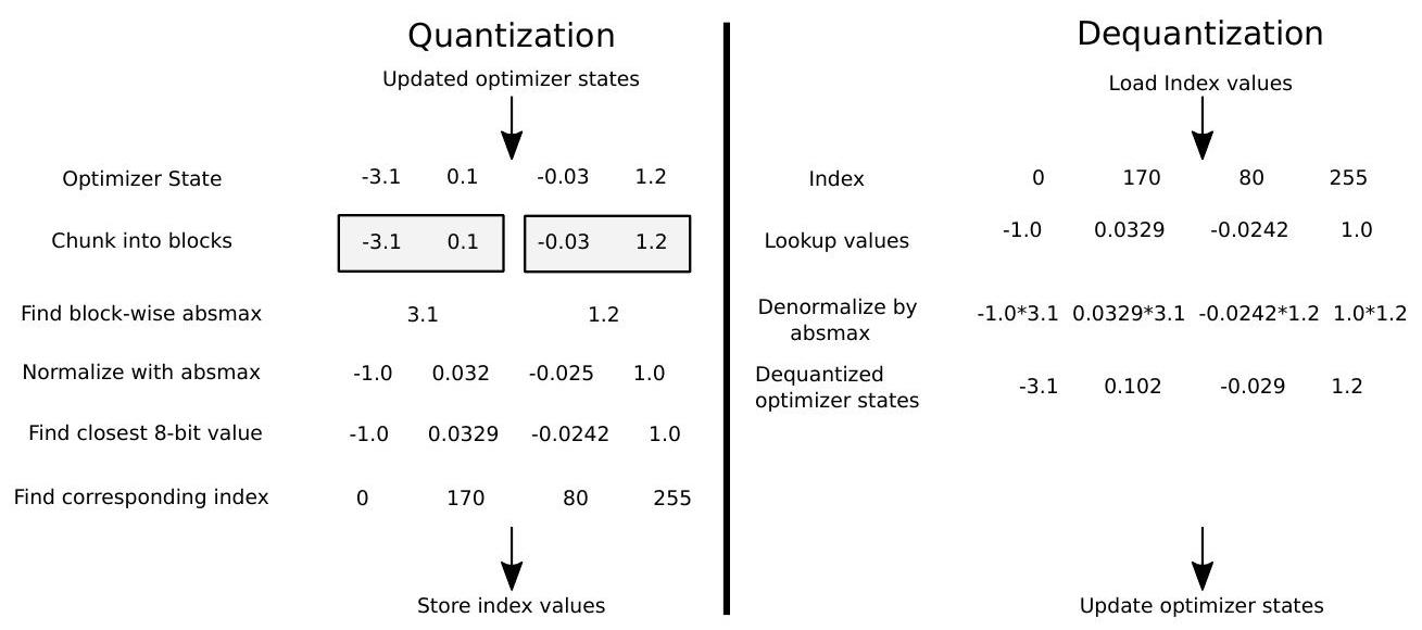
Figure 1: Schematic of 8-bit optimizers via block-wise dynamic quantization, see Section 2 for more details. After the optimizer update is performed in 32-bit, the state tensor is chunked into blocks, normalized by the absolute maximum value of each block. Then dynamic quantization is performed, and the index is stored. For dequantization, a lookup in the index is performed, with subsequent denormalization by multiplication with the block-wise absolute maximum value. Outliers are confined to a single block through block-wise quantization, and their effect on normalization is limited.

图 1：通过逐块动态量化的 8 位优化器示意图，有关更多详细信息，请参阅第 2 节。 在 32 位执行优化器更新后，状态张量被分成块，由每个块的绝对最大值归一化。 然后进行动态量化，并存储索引。 对于反量化，执行索引中的查找，随后通过与块级绝对最大值相乘来进行反规范化。 通过逐块量化将异常值限制在单个块中，并且它们对归一化的影响有限。

and rare large ones. However, to be practical, 8-bit optimizers need to be fast enough to not slow down training, which is especially difficult for non-linear methods that require more complex data structures to maintain the quantization buckets. Finally, to maintain stability with huge models beyond 1B parameters, a quantization method needs to not only have a good mean error but excellent worse case performance since a single large quantization error can cause the entire training run to diverge.

然而，为了实用，8 Bit 优化器需要足够快才能不减慢训练速度，这对于需要更复杂的数据结构来维护量化桶的非线性方法来说尤其困难。最后，为了保持超过 1B 参数的大型模型的稳定性，量化方法不仅需要具有良好的平均误差，而且还需要具有出色的最坏情况性能，因为单个较大的量化误差会导致整个训练运行发散。

We introduce a new block-wise quantization approach that addresses all three of these challenges. Block-wise quantization splits input tensors into blocks and performs quantization on each block independently. This block-wise division reduces the effect of outliers on the quantization process since they are isolated to particular blocks, thereby improving stability and performance, especially for large-scale models. Block-wise processing also allows for high optimizer throughput since each normalization can be computed independently in each core. This contrasts with tensor-wide normalization, which requires slow cross-core synchronization that is highly dependent on task-core scheduling. We combine block-wise quantization with two novel methods for stable, high-performance 8-bit optimizers: dynamic quantization and a stable embedding layer. Dynamic quantization is an extension of dynamic tree quantization for unsigned input data. The stable embedding layer is a variation of a standard word embedding layer that supports more aggressive quantization by normalizing the highly non-uniform distribution of inputs to avoid extreme gradient variation.

我们引入了一种新的逐块量化方法来解决所有这三个挑战。逐块量化将输入张量分成块，并对每个块独立执行量化。这种逐块划分减少了异常值对量化过程的影响，因为它们与特定块隔离，从而提高了稳定性和性能，尤其是对于大规模模型。逐块处理还允许优化器的高吞吐量，因为每个规范化都可以在每个内核中独立计算。这与张量范围的标准化形成对比，后者需要高度依赖于任务CPU 核心调度的缓慢的跨CPU 核心同步。我们将逐块量化与两种用于稳定、高性能 8 Bit 优化器的新方法相结合：动态量化和稳定嵌入层。动态量化是对无符号输入数据的动态树量化的扩展。稳定嵌入层是标准词嵌入层的变体，它通过对输入的高度不均匀分布进行归一化来支持更积极的量化，以避免极端的梯度变化。

Our 8-bit optimizers maintain 32-bit performance at a fraction of the original memory footprint. We show this for a broad range of tasks: 1.5B and 355M parameter language modeling, GLUE finetuning, ImageNet classification, WMT'14+WMT' 16 machine translation, MoCo v2 contrastive image pretraining+finetuning, and RoBERTa pretraining. We also report additional ablations and sensitivity analysis showing that all components - block-wise quantization, dynamic quantization, and stable embedding layer - are crucial for these results and that 8-bit Adam can be used as a simple drop-in replacement for 32-bit Adam, with no hyperparameter changes. We open-source our custom CUDA kernels and provide a PyTorch implementation that enables 8-bit optimization by changing two lines of code.

我们的 8 Bit 优化器以原始内存占用的一小部分保持 32 Bit 性能。我们针对广泛的任务展示了这一点：1.5B 和 355M 参数语言建模、GLUE 微调、ImageNet 分类、WMT'14+WMT'16 机器翻译、MoCo v2 对比图像预训练+微调和 RoBERTa 预训练。我们还报告了额外的消融和灵敏度分析，表明所有组件 - 逐块量化、动态量化和稳定嵌入层 - 对于这些结果至关重要，并且 8 Bit Adam 可以用作 32- 的简单替代品Bit Adam，没有改变超参数。我们将自定义 CUDA 内核开源，并提供 PyTorch 实现，通过更改两行代码即可实现 8 Bit 优化。

BACKGROUND

Stateful Optimizers

An optimizer updates the parameters w of a neural network by using the gradient of the loss with respect to the weight $\mathbf{g}_{t}=\frac{\partial \mathbf{L} }{\partial \mathbf{w} }$ at update iteration $t$. Stateful optimizers compute statistics of the gradient with respect to each parameter over time for accelerated optimization. Two of the most commonly used stateful optimizers are Adam (Kingma and Ba, 2014), and SGD with momentum (Qian, 1999) - or Momentum for short. Without damping and scaling constants, the update rules of these optimizers are given by:

优化器通过使用损失相对于权重的梯度 $\mathbf{g}{t}=\frac{\partial \mathbf{L} }{\partial \mathbf{w} }$ 来更新神经网络的参数 w. 有状态优化器随时间计算每个参数的梯度统计数据，以加速优化。两个最常用的有状态优化器是 Adam（Kingma 和 Ba，2014 年）和带动量的 SGD（Qian，1999 年）——或简称 Momentum。在没有阻尼和缩放常数的情况下，这些优化器的更新规则由下式给出： $$ \begin{gathered} \operatorname{Momentum}\left(\mathbf{g}, \mathbf{w}{t-1}, \mathbf{m}\right)= \begin{cases}\mathbf{m}{0}=\mathbf{g} & \text { Initialization } \ \mathbf{m}{t}=\beta \mathbf{m}{t-1}+\mathbf{g} & \text { State 1 update } \ \mathbf{w}{t}=\mathbf{w}-\alpha \cdot \mathbf{m}{t} & \text { Weight update }\end{cases} \ \operatorname{Adam}\left(\mathbf{g}, \mathbf{w}{t-1}, \mathbf{m}, \mathbf{r}{t-1}\right)= \begin{cases}\mathbf{r}=\mathbf{m}{0}=\mathbf{0} & \text { Initialization } \ \mathbf{m}=\beta_{1} \mathbf{m}{t-1}+\left(1-\beta\right) \mathbf{g}{t} & \text { State 1 update } \ \mathbf{r}=\beta_{2} \mathbf{r}{t-1}+\left(1-\beta\right) \mathbf{g}{t}^{2} & \text { State 2 update } \ \mathbf{w}=\mathbf{w}{t-1}-\alpha \cdot \frac{\mathbf{m} }{\sqrt{\mathbf{r}_{t} }+\epsilon} & \text { Weight update, }\end{cases} \end{gathered} $$

where $\beta_{1}$ and $\beta_{2}$ are smoothing constants, $\epsilon$ is a small constant, and $\alpha$ is the learning rate.

For 32-bit states, Momentum and Adam consume 4 and 8 bytes per parameter. That is 4 GB and 8 GB for a 1B parameter model. Our 8-bit non-linear quantization reduces these costs to $1 \mathrm{~GB}$ and 2 GB.

对于 32 Bit 状态，Momentum 和 Adam 每个参数消耗 4 和 8 个字节。对于 1B 参数模型，即 4 GB 和 8 GB。我们的 8 Bit 非线性量化将这些成本降低到1 GB 和 2 GB。

NON-Linear Quantization

Quantization compresses numeric representations to save space at the cost of precision. Quantization is the mapping of a $k$-bit integer to a real element in $D$, that is, $\mathbf{Q}^{\text {map } }:\left[0,2^{k}-1\right] \mapsto D$. For example, the IEEE 32-bit floating point data type maps the indices $0 \ldots 2^{32}-1$ to the domain $[-3.4 \mathrm{e} 38,+3.4 \mathrm{e} 38]$. We use the following notation: $\mathbf{Q}^{\text {map } }(i)=\mathbf{Q}{i}^{\text {map } }=q$, for example $\mathbf{Q}^{\text {map } }\left(2^{31}+131072\right)=2.03125$, for the IEEE 32-bit floating point data type.

To perform general quantization from one data type into another we require three steps. (1) Compute a normalization constant $N$ that transforms the input tensor $\mathbf{T}$ into the range of the domain $D$ of the target quantization data type $\mathbf{Q}^{\text {map } }$, (2) for each element of $\mathbf{T} / N$ find the closest corresponding value $q_{i}$ in the domain $D$, (3) store the index $i$ corresponding to $q_{i}$ in the quantized output tensor $\mathbf{T}^{Q}$. To receive the dequantized tensor $\mathbf{T}^{D}$ we look up the index and denormalize: $\mathbf{T}{i}^{D}=\mathbf{Q}^{\text {map } }\left(\mathbf{T}^{Q}\right) \cdot N$.

To perform this procedure for dynamic quantization we first normalize into the range $[-1,1]$ through division by the absolute maximum value: $N=\max (|\mathbf{T}|)$.

Then we find the closest values via a binary search:

$$ \mathbf{T}{i}^{Q}=\underset{j=0}{\stackrel{2^{n} }{\arg \min } }\left|\mathbf{Q}^{\mathrm{map} }-\frac{\mathbf{T}_{i} }{N}\right| $$

Dynamic Tree Quantization

Dynamic Tree quantization (Dettmers, 2016) is a method that yields low quantization error for both small and large magnitude values. Unlike data types with fixed exponent and fraction, dynamic tree quantization uses a datatype with a dynamic exponent and fraction that can change with each number. It is made up of four parts, as seen in Figure 2 (1) The first bit of the data type is reserved for a sign. (2) The number of subsequent zero bits indicates the magnitude of the exponent. (3) The first bit that is set to one indicates that all following values are reserved for (4) linear quantization. By moving the indicator bit, numbers can have a large exponent $10^{-7}$ or precision as high as $1 / 63$. Compared to linear quantization, dynamic tree quantization has better absolute and relative quantization errors for non-uniform distributions. Dynamic tree quantization is strictly defined to quantize numbers in the range $[-1.0,1.0]$, which is ensured by performing tensor-level absolute max normalization.

动态树量化 (Dettmers, 2016) 是一种对小值和大值都产生低量化误差的方法。与具有固定指数和分数的数据类型不同，动态树量化使用具有随每个数字变化的动态指数和分数的数据类型。它由四部分组成，如图 2 (1) 数据类型的第一位保留为符号。(2) 后续零位 的个数表示指数的大小。(3) 设置为 1 的第一位 表示以下所有值都保留给(4)线性量化。通过移动指示位 ，数字可以有一个大的指数10−7或精度高达1/63. 与线性量化相比，动态树量化对于非均匀分布具有更好的绝对和相对量化误差。动态树量化被严格定义为量化范围内的数字[−1.0,1.0][−1.0,1.0]，这是通过执行张量级绝对最大归一化来确保的。

Figure 2: Dynamic tree quantization.

8-BIT OPTIMIZERS

Our 8-bit optimizers have three components: (1) block-wise quantization that isolates outliers and distributes the error more equally over all bits; (2) dynamic quantization, which quantizes both small and large values with high precision; and (3) a stable embedding layer to improve stability during optimization for models with word embeddings.

With these components, performing an optimizer update with 8-bit states is straightforward. We dequantize the 8-bit optimizer states to 32-bit, perform the update, and then quantize the states back to 8-bit for storage. We do this 8-bit to 32-bit conversion element-by-element in registers, which means no slow copies to GPU memory or additional temporary memory are needed to perform quantization and dequantization. For GPUs, this makes 8-bit optimizers faster than regular 32-bit optimizers, as we show in Section 3

我们的 8 Bit 优化器包含三个组件：(1) 逐块量化，隔离异常值并在所有Bit 上更平均地分配错误；(2) 动态量化，对小值和大值都进行高精度量化；(3) 一个稳定的嵌入层，以提高具有词嵌入的模型优化过程中的稳定性。

使用这些组件，使用 8 Bit 状态执行优化器更新非常简单。我们将 8 Bit 优化器状态反量化为 32 Bit ，执行更新，然后将状态量化回 8 Bit 以进行存储。我们在寄存器中逐个元素地执行这种 8 Bit 到 32 Bit 的转换，这意味着不需要慢速复制到 GPU 内存或额外的临时内存来执行量化和反量化。对于 GPU，这使得 8 Bit 优化器比常规的 32 Bit 优化器更快，正如我们在第 3 节中展示的那样

BLOCK-WISE QUANTIZATION

Our block-wise quantization reduces the cost of computing normalization and improves quantization precision by isolating outliers. In order to dynamically quantize a tensor, as defined in Section 1.2 we need to normalize the tensor into the range $[-1,1]$. Such normalization requires a reduction over the entire tensor, which entails multiple synchronizations across GPU cores. Block-wise dynamic quantization reduces this cost by chunking an input tensor into small blocks of size $B=2048$ and performing normalization independently in each core across this block.

我们的逐块量化降低了计算归一化的成本，并通过隔离异常值提高了量化精度。为了动态量化张量，如第 1.2 节中所定义，我们需要将张量归一化到 $[-1,1]$ 范围内. 这种规范化需要对整个张量进行缩减，这需要跨 GPU 内核进行多次同步。逐块动态量化通过将输入张量分块为$B=2048$小块来降低成本， 并在该块的每个CPU 核心中独立执行归一化。

More formally, using the notation introduced in Section 1.2 in block-wise quantization, we treat $\mathbf{T}$ as a one-dimensional sequence of elements that we chunk in blocks of size $B$. This means for an input tensor $\mathbf{T}$ with $n$ elements we have $n / B$ blocks. We proceed to compute a normalization constant for each block: $N_{b}=\max \left(\left|\mathbf{T}_{b}\right|\right)$, where $b$ is the index of the block $0 . . n / B$. With this block-wise normalization constant, each block can be quantized independently:

更正式地说，使用 1.2 节中介绍的逐块量化符号，我们将 $\mathbf{T}$ 作为一个一维的元素序列，我们将其分成大小块$B$ 这意味着对于输入$n$ 元素 的张量 $\mathbf{T}$ , 我们拥有 $n / B$ 个块。我们继续为每个块计算归一化常数：$N_{b}=\max \left(\left|\mathbf{T}{b}\right|\right)$， 其中 $b$ 是块的索引 $0 . . n / B$. 使用这个逐块归一化常数，每个块都可以独立量化： $$ \mathbf{T}^{Q}=\left.\underset{j=0}{\arg \min }\left|\mathbf{Q}{j}^{\text {map } }-\frac{\mathbf{T} }{N_{b} }\right|\right|_{0<i<B} $$

This approach has several advantages, both for stability and efficiency. First, each block normalization can be computed independently. Thus no synchronization between cores is required, and throughput is enhanced.

这种方法在稳定性和效率方面都有几个优点。首先，每个块归一化都可以独立计算。因此不需要CPU 核心之间的同步，并且提高了吞吐量。

Secondly, it is also much more robust to outliers in the input tensor. For example, to contrast blockwise and regular quantization, if we create an input tensor with one million elements sampled from the standard normal distribution, we expect less than $1 %$ of elements of the tensor will be in the range $[3,+\infty)$. However, since we normalize the input tensor into the range $[-1,1]$ this means the maximum values of the distribution determine the range of quantization buckets. This means if the input tensor contains an outlier with magnitude 5 , the quantization buckets reserved for numbers between 3 and 5 will mostly go unused since less than $1 %$ of numbers are in this range. With blockwise quantization, the effect of outliers is limited to a single block. As such, most bits are used effectively in other blocks.

其次，它对输入张量中的异常值也更加稳健。例如，为了对比分块量化和常规量化，如果我们创建一个包含从标准正态分布中采样的一百万个元素的输入张量，我们期望少于1%张量的元素将在[3,+∞)范围内. 然而，由于我们将输入张量归一化到 [−1,1] 范围内。 这意味着分布的最大值决定了量化桶的范围。这意味着如果输入张量包含一个幅度为 5 的异常值，则为 3 到 5 之间的数字保留的量化桶将大部分未使用，因为小于1% 的数字在这个范围内。使用分块量化，异常值的影响仅限于单个块。因此，大多数Bit 在其他块中得到有效使用。

Furthermore, because outliers represent the absolute maximum value in the input tensor, blockwise quantization approximates outlier values without any error. This guarantees that the largest optimizer states, arguably the most important, will always be quantized with full precision. This property makes block-wise dynamic quantization both robust and precise and is essential for good training performance in practice.

此外，因为离群值代表输入张量中的绝对最大值，所以分块量化近似于离群值而没有任何错误。这保证了最大的优化器状态，可以说是最重要的，将始终以完全精确的方式进行量化。此属性使逐块动态量化既稳健又精确，并且对于实践中的良好训练性能至关重要。

DYNAmiC QuAntization

In this work, we extend dynamic tree quantization (Section 1.3 for non-signed input tensors by re-purposing the sign bit. Since the second Adam state is strictly positive, the sign bit is not needed. Instead of just removing the sign bit, we opt to extend dynamic tree quantization with a fixed bit for the fraction. This extension is motivated by the observation that the second Adam state varies around 3-5 orders of magnitude during the training of a language model. In comparison, dynamic tree quantization already has a range of 7 orders of magnitude. We refer to this quantization as dynamic quantization to distinguish it from dynamic tree quantization in our experiments. A study of additional quantization data types and their performance is detailed in Appendix F

在这项工作中，我们通过重新调整符号Bit 来扩展动态树量化（第 1.3 节，针对无符号输入张量）。由于第二个 Adam 状态严格为正，因此不需要符号Bit 。而不是仅仅删除符号Bit ，我们选择使用分数的固定Bit 来扩展动态树量化。这种扩展的动机是观察到在语言模型的训练过程中，第二个 Adam 状态变化大约 3-5 个数量级。相比之下，动态树量化已经具有 7 个数量级的范围。我们将这种量化称为动态量化，以区别于我们实验中的动态树量化。附加量化数据类型及其性能的研究详见附录 F

Stable Embedding LAYer

Our stable embedding layer is a standard word embedding layer variation (Devlin et al., 2019) designed to ensure stable training for NLP tasks. This embedding layer supports more aggressive quantization by normalizing the highly non-uniform distribution of inputs to avoid extreme gradient variation. See Appendix $\mathrm{C}$ for a discussion of why commonly adopted embedding layers (Ott et al. 2019) are so unstable.

我们的稳定嵌入层是标准的词嵌入层变体（Devlin 等人，2019 年），旨在确保 NLP 任务的稳定训练。该嵌入层通过对输入的高度不均匀分布进行归一化来支持更积极的量化，以避免极端的梯度变化。参见附录C讨论为什么普遍采用的嵌入层 (Ott et al. 2019) 如此不稳定。

We initialize the Stable Embedding Layer with Xavier uniform initialization (Glorot and Bengio, 2010) and apply layer normalization (Ba et al., 2016) before adding position embeddings. This method maintains a variance of roughly one both at initialization and during training. Additionally, the uniform distribution initialization has less extreme values than a normal distribution, reducing maximum gradient size. Like Ramesh et al. (2021), we find that the stability of training improves significantly if we use 32-bit optimizer states for the embedding layers. This is the only layer that uses 32-bit optimizer states. We still use the standard precision for weights and gradients for the embedding layers - usually 16-bit. We show in our Ablation Analysis in Section 4 that the Stable Embedding Layer is required for stable training. See ablations for the Xavier initialization, layer norm, and 32-bit state components of the Stable Embedding Layer in Appendix I.

我们使用 Xavier 统一初始化 (Glorot and Bengio, 2010) 初始化稳定嵌入层，并在添加Bit 置嵌入之前应用层归一化 (Ba et al., 2016)。这种方法在初始化和训练期间都保持大约为 1 的方差。此外，均匀分布初始化具有比正态分布更少的极值，从而减小了最大梯度大小。像 Ramesh 等人。(2021)，我们发现如果我们对嵌入层使用 32 Bit 优化器状态，训练的稳定性会显着提高。这是唯一使用 32 Bit 优化器状态的层。我们仍然对嵌入层的权重和梯度使用标准精度——通常是 16 Bit 。我们在第 4 节的消融分析中表明，稳定的嵌入层是稳定训练所必需的。

8-Bit vs 32-Bit Optimizer PERformanCE FOR COMMON BenCHMARKS

Experimental Setup

We compare the performance of 8-bit optimizers to their 32-bit counterparts on a range of challenging public benchmarks. These benchmarks either use Adam (Kingma and $\mathrm{Ba}$ 2014), AdamW (Loshchilov and Hutter, 2018), or Momentum (Qian, 1999).

我们比较了 8 Bit 优化器与 32 Bit 优化器在一系列具有挑战性的公共基准测试中的性能。这些基准测试要么使用 Adam（Kingma 和乙A不是2014)、AdamW（Loshchilov 和 Hutter，2018）或 Momentum（Qian，1999）。

We do not change any hyperparameters or precision of weights, gradients, and activations/input gradients for each experimental setting compared to the public baseline- the only change is to replace 32-bit optimizers with 8-bit optimizers. This means that for most experiments, we train in 16-bit mixed-precision (Micikevicius et al., 2017). We also compare with Adafactor (Shazeer and Stern. 2018), with the time-independent formulation for $\beta_{2}$ (Shazeer and Stern 2018) - which is the same formulation used in Adam. We also do not change any hyperparameters for Adafactor.

与公共基线相比，我们不会更改每个实验设置的任何超参数或权重、梯度和激活/输入梯度的精度——唯一的变化是用 8 Bit 优化器替换 32 Bit 优化器。这意味着对于大多数实验，我们以 16 Bit 混合精度进行训练（Micikevicius 等人，2017 年）。我们还与 Adafactor（Shazeer 和 Stern。2018）进行了比较，其中时间无关的公式为$\beta_{2}$（Shazeer 和 Stern 2018）——这与 Adam 中使用的公式相同。我们也不更改 Adafactor 的任何超参数。

We report on benchmarks in neural machine translation $\sqrt{\text { Ott et al., } 2018 |^{2} }$ trained on WMT'16 (Sennrich et al., 2016) and evaluated on en-de WMT'14 (Macháček and Bojar. 2014), large-scale language modeling (Lewis et al. 2021; Brown et al., 2020) and RoBERTa pretraining (Liu et al. 2019) on English CC-100 + RoBERTa corpus (Nagel. 2016; Gokaslan and Cohen. 2019. Zhu et al. 2015: Wenzek et al. 2020), finetuning the pretrained masked language model RoBERTa (Liu et al. $2019)^{3}$ on GLUE (Wang et al., 2018a), ResNet-50 v1.5 image classification (He et al. 2016. ImageNet-1k (Deng et al., 2009), and Moco v2 contrastive image pretraining and linear finetuning Chen et al. 2020b ${ }^{5}$ on ImageNet-1k (Deng et al. 2009).

我们报告了神经机器翻译的基准，在 WMT'16（Sennrich 等人，2016 年）上接受训练并在 en-de WMT'14（Macháček 和 Bojar。2014 年）、大规模语言建模（Lewis 等人，2021 年；Brown 等人，2020 年）和RoBERTa pretraining (Liu et al. 2019) on English CC-100 + RoBERTa corpus (Nagel. 2016; Gokaslan and Cohen. 2019. Zhu et al. 2015: Wenzek et al. 2020)，微调预训练掩码语言模型 RoBERTa (Liu等。2019)32019)3关于 GLUE（Wang et al., 2018a）、ResNet-50 v1.5 图像分类（He et al. 2016. ImageNet-1k（Deng et al., 2009）和 Moco v2 对比图像预训练和线性微调 Chen 等人. 2020b55 on ImageNet-1k (Deng et al. 2009).

We use the stable embedding layer for all NLP tasks except for finetuning on GLUE. Beyond this, we follow the exact experimental setup outlined in the referenced papers and codebases. We consistently report replication results for each benchmark with public codebases and report median accuracy, perplexity, or BLEU over ten random seeds for GLUE, three random seeds for others tasks, and a single random seed for large scale language modeling. While it is standard to report means and standard errors on some tasks, others use median performance. We opted to report medians for all tasks for consistency.

除了 GLUE 上的微调外，我们对所有 NLP 任务都使用稳定的嵌入层。除此之外，我们遵循参考论文和代码库中概述的确切实验设置。我们始终如一地报告具有公共代码库的每个基准测试的复制结果，并报告 GLUE 的十个随机种子的中值准确度、困惑度或 BLEU，其他任务的三个随机种子和大规模语言建模的单个随机种子。虽然报告某些任务的均值和标准误差是标准的，但其他任务使用中Bit 数表现。我们选择报告所有任务的中Bit 数以保持一致性。

Results In Table1, we see that 8-bit optimizers match replicated 32-bit performance for all tasks. While Adafactor is competitive with 8-bit Adam, 8-bit Adam uses less memory and provides faster optimization. Our 8-bit optimizers save up to 8.5 GB of GPU memory for our largest 1.5B pa-

Table 1: Median performance on diverse NLP and computer vision tasks: GLUE, object classification with (Moco v2) and without pretraining (CLS), machine translation (MT), and large-scale language modeling (LM). While 32-bit Adafactor is competitive with 8-bit Adam, it uses almost twice as much memory and trains slower. 8-bit Optimizers match or exceed replicated 32-bit performance on all tasks. We observe no instabilities for 8-bit optimizers. Time is total GPU time on V100 GPUs, except for RoBERTa and GPT3 pretraining, which were done on A100 GPUs.

结果 在表 1 中，我们看到 8 Bit 优化器匹配所有任务的复制 32 Bit 性能。虽然 Adafactor 与 8 Bit Adam 竞争，但 8 Bit Adam 使用更少的内存并提供更快的优化。我们的 8 Bit 优化器为我们最大的 1.5B 参数语言模型和 2.0 GB 用于 RoBERTa节省了高达 8.5 GB 的 GPU 内存 。 因此，8 Bit 优化器保持性能并提高那些买不起 GPU 的人对大型模型进行微调的可访问性通过大内存缓冲区。 我们在表 2 中展示了现在可以使用较小 GPU 访问的模型。 可以在附录 B 中找到 GLUE 上单个数据集结果的细分）。

广泛的任务和竞争结果表明，8 Bit 优化器是 32 Bit 优化器的强大而有效的替代品，不需要对超参数进行任何额外更改，并且在略微加快训练速度的同时节省了大量内存。

表 1：各种 NLP 和计算机视觉任务的中值性能：GLUE、使用 (Moco v2) 和不使用预训练 (CLS) 的对象分类、机器翻译 (MT) 和大规模语言建模 (LM)。虽然 32 Bit Adafactor 与 8 Bit Adam 具有竞争力，但它使用的内存几乎是其两倍，而且训练速度更慢。8 Bit 优化器在所有任务上均达到或超过复制的 32 Bit 性能。我们没有观察到 8 Bit 优化器的不稳定性。时间是 V100 GPU 上的总 GPU 时间，RoBERTa 和 GPT3 预训练除外，它们是在 A100 GPU 上完成的。

††指标：GLUE=平均准确度/相关性。CLS/MoCo = 准确度。MT=蓝色。LM=困惑。

表 2：与标准 32 Bit 优化器训练相比，使用 8 Bit 优化器可以使用相同的 GPU 内存对更大的模型进行微调。我们使用批量大小 1 进行比较。

${ }^{\dagger}$ Metric: GLUE=Mean Accuracy/Correlation. CLS/MoCo = Accuracy. MT=BLEU. LM=Perplexity.

rameter language model and 2.0 GB for RoBERTa. Thus, 8-bit optimizers maintain performance and improve accessibility to the finetuning of large models for those that cannot afford GPUs with large memory buffers. We show models that are now accessible with smaller GPUs in Table 2 A breakdown of individual dataset results on GLUE can be found in Appendix B.

The broad range of tasks and competitive results demonstrate that 8-bit optimizers are a robust and effective replacement for 32-bit optimizers, do not require any additional changes in hyperparameters, and save a significant amount of memory while speeding up training slightly.

Table 2: With 8-bit optimizers, larger models can be finetuned with the same GPU memory compared to standard 32-bit optimizer training. We use a batch size of one for this comparison.

ANALYSIS

We analyze our method in two ways. First, we ablate all 8-bit optimizer components and show that they are necessary for good performance. Second, we look at the sensitivity to hyperparameters compared to 32-bit Adam and show that 8-bit Adam with block-wise dynamic quantization is a reliable replacement that does not require further hyperparameter tuning.

我们以两种方式分析我们的方法。首先，我们消除了所有 8 Bit 优化器组件，并表明它们是获得良好性能所必需的。其次，我们比较了 32 Bit Adam 对超参数的敏感性，并表明具有块动态量化的 8 Bit Adam 是一种可靠的替代品，不需要进一步的超参数调整。

Experimental Setup We perform our analysis on a strong 32-bit Adam baseline for language modeling with transformers (Vaswani et al., 2017). We subsample from the RoBERTa corpus (Liu et al. 2019) which consists of the English sub-datasets: Books (Zhu et al., 2015), Stories (Trinh and Le.|2018), OpenWebText-1 (Gokaslan and Cohen, 2019), Wikipedia, and CC-News (Nagel. 2016). We use a 50k token BPE encoded vocabulary (Sennrich et al., 2015). We find the best 2-GPU-day transformer baseline for 32-bit Adam with multiple hyperparameter searches that take in a total of 440 GPU days. Key hyperparameters include 10 layers with a model dimension of 1024, a fully connected hidden dimension of 8192, 16 heads, and input sub-sequences with a length of 512 tokens each. The final model has $209 \mathrm{~m}$ parameters.

实验设置

我们在强大的 32 Bit Adam 基线上执行我们的分析，用于使用转换器进行语言建模（Vaswani 等人，2017）。我们从 RoBERTa 语料库 (Liu et al. 2019) 中抽样，该语料库由英语子数据集组成：Books (Zhu et al., 2015)、Stories (Trinh and Le.|2018)、OpenWebText-1 (Gokaslan and Cohen, 2019)、维基百科和 CC-News (Nagel. 2016)。我们使用 50k 令牌的 BPE 编码词汇表（Sennrich 等人，2015 年）。我们通过多个超参数搜索找到了 32 Bit Adam 的最佳 2-GPU-day 转换器基线，总共花费了 440 GPU 天。关键超参数包括 10 层，模型维度为 1024，完全连接的隐藏维度为 8192，16 个头，以及每个长度为 512 个Token的输入子序列。最终模型有209 M参数。

Table 3: Ablation analysis of 8-bit Adam for small (2 GPU days) and large-scale ( $\approx 1$ GPU year) transformer language models on the RoBERTa corpus. The runs without dynamic quantization use linear quantization. The percentage of unstable runs indicates either divergence or crashed training due to exploding gradients. We report median perplexity for successful runs. We can see that dynamic quantization is critical for general stability and block-wise quantization is critical for largescale stability. The stable embedding layer is useful for both 8-bit and 32-bit Adam and enhances stability to some degree.

表 3：针对小型（2 GPU 天）和大规模（≈1GPU 年）RoBERTa 语料库上的变换器语言模型。没有动态量化的运行使用线性量化。不稳定运行的百分比表示由于梯度爆炸导致的分歧或崩溃训练。我们报告成功运行的中Bit 困惑。我们可以看到，动态量化对于一般稳定性至关重要，而逐块量化对于大规模稳定性至关重要。稳定嵌入层对 8 Bit 和 32 Bit Adam 都有用，并在一定程度上增强了稳定性。

Ablation Analysis For the ablation analysis, we compare small and large-scale language modeling perplexity and training stability against a 32-bit Adam baseline. We ablate components individually and include combinations of methods that highlight their interactions. The baseline method uses linear quantization, and we add dynamic quantization, block-wise quantization, and the stable embedding layer to demonstrate their effect. To test optimization stability for small-scale language modeling, we run each setting with different hyperparameters and report median performance across all successful runs. A successful run is a run that does not crash due to exploding gradients or diverges in the loss. We use the hyperparameters $\epsilon{1 \mathrm{e}-8,1 \mathrm{e}-7,1 \mathrm{e}-6}, \beta_{1}{0.90,0.87,0.93}, \beta_{2}$ ${0.999,0.99,0.98}$ and small changes in learning rates. We also include some partial ablations for large-scale models beyond 1B parameters. In the large-scale setting, we run several seeds with the same hyperparameters. We use a single seed for 32-bit Adam, five seeds for 8-bit Adam at 1.3B parameters, and a single seed for 8-bit Adam at 1.5B parameters ${ }^{6}$ Results are shown in Table 3.

消融分析

对于消融分析，我们将小型和大型语言建模的困惑度和训练稳定性与 32 Bit Adam 基线进行了比较。我们单独消融组件，并包括突出它们交互的方法组合。基线方法使用线性量化，我们添加动态量化、逐块量化和稳定嵌入层来演示它们的效果。为了测试小规模语言建模的优化稳定性，我们使用不同的超参数运行每个设置，并报告所有成功运行的中值性能。成功的运行是不会因梯度爆炸或损失发散而崩溃的运行。我们使用超参数 $\epsilon{1 \mathrm{e}-8,1 \mathrm{e}-7,1 \mathrm{e}-6}, \beta_{1}{0.90,0.87,0.93}, \beta_{2}$ ${0.999,0.99,0.98}$ 和学习率的微小变化。我们还包括一些超过 1B 参数的大型模型的部分消融。在大规模设置中，我们使用相同的超参数运行多个种子。我们对 32 Bit Adam 使用单个种子，对 1.3B 参数的 8 Bit Adam 使用五个种子，对 1.5B 参数的 8 Bit Adam 使用单个种子66结果如表 3 所示。

The Ablations show that dynamic quantization, block-wise quantization, and the stable embedding layer are critical for either performance or stability. In addition, block-wise quantization is critical for large-scale language model stability.

Sensitivity Analysis We compare the perplexity of 32-bit Adam vs 8-bit Adam + Stable Embedding as we change the optimizer hyperparameters: learning rate, betas, and $\epsilon$. We change each hyperparameter individually from the baseline hyperparameters $\beta_{1}=0.9, \beta_{2}=0.995, \epsilon=1 \mathrm{e}-7$, and $\mathrm{lr}=0.0163$

消融表明动态量化、逐块量化和稳定的嵌入层对于性能或稳定性都至关重要。此外，逐块量化对于大规模语言模型的稳定性至关重要。

敏感性分析

我们比较了 32 Bit Adam 与 8 Bit Adam + 稳定嵌入的困惑度，因为我们改变了优化器的超参数：学习率、beta 和ε. 我们从基线超参数中单独更改每个超参数$\beta_{1}=0.9, \beta_{2}=0.995, \epsilon=1 \mathrm{e}-7$, and $\mathrm{lr}=0.0163$并为每个设置为 8 Bit 和 32 Bit Adam 运行两个随机种子。如果与 32 Bit Adam 相比，8 Bit Adam 对超参数完全不敏感，那么我们预计任何超参数组合的性能都会有相同的常数偏移。结果如图 3 所示，结果显示 8 Bit 和 32 Bit Adam 之间存在相对稳定的差距，这表明与 32 Bit Adam 相比，8 Bit Adam 不需要任何进一步的超参数调整。

${ }^{6}$ We chose not to do the full ablations with such large models because each training run takes one GPU year. and run two random seeds for both 8-bit and 32-bit Adam for each setting. If 8-bit Adam is perfectly insensitive to hyperparameters compared to 32-bit Adam, we would expect the same constant offset in performance for any hyperparameter combination. The results can be seen in Figure 3 The results show a relatively steady gap between 8-bit and 32-bit Adam, suggesting that 8-bit Adam does not require any further hyperparameter tuning compared to 32-bit Adam.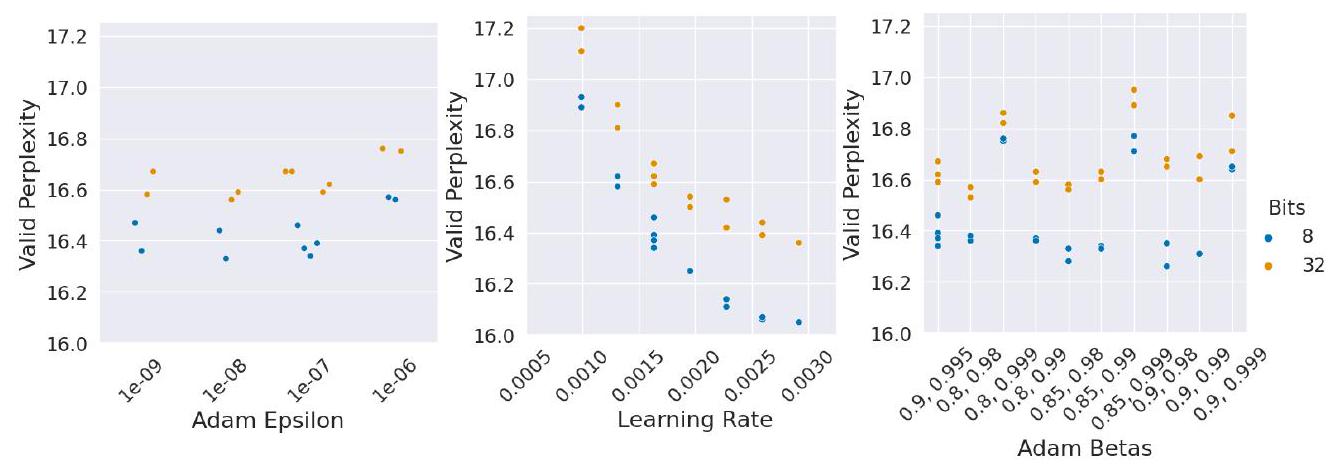

Figure 3: Sensitivity analysis of 8-bit vs 32-bit Adam hyperparameters. We can see that there is little variance between 8 and 32-bit performance, which suggests that 8-bit Adam can be used as a drop-in replacement for 32-bit Adam without any further hyperparameter tuning.

图 3：8 Bit 与 32 Bit Adam 超参数的灵敏度分析。我们可以看到 8 Bit 和 32 Bit 性能之间几乎没有差异，这表明 8 Bit Adam 可以用作 32 Bit Adam 的直接替代品，无需任何进一步的超参数调整。

RELATED WORK

Compressing & Distributing Optimizer States While 16-bit Adam has been used in several publications, the stability of 16-bit Adam was first explicitly studied for a text-to-image generation model DALL-E (Ramesh et al. 2021). They show that a stable embedding layer, tensor-wise scaling constants for both Adam states, and multiple loss scaling blocks are critical to achieving stability during training. Our work reduces the memory footprint of Adam further, from 16 to 8-bit. In addition, we achieve stability by developing new training procedures and non-linear quantization, both of which complement previous developments.

压缩和分布式优化器状态

虽然 16 Bit Adam 已在多个出版物中使用，但首先针对文本到图像生成模型 DALL-E 明确研究了 16 Bit Adam 的稳定性（Ramesh 等人，2021 年）。他们表明，稳定的嵌入层、两个 Adam 状态的张量缩放常数和多个损失缩放块对于在训练期间实现稳定性至关重要。我们的工作进一步减少了 Adam 的内存占用，从 16 Bit 减少到 8 Bit 。此外，我们通过开发新的训练程序和非线性量化来实现稳定性，这两者都是对先前发展的补充。

Adafactor (Shazeer and Stern, 2018) uses a different strategy to save memory. All optimizer states are still 32-bit, but the second Adam state is factorized by a row-column outer product resulting in a comparable memory footprint to 16-bit Adam. Alternatively, Adafactor can also be used without using the first moment $\left(\beta_{1}=0.0\right)$ (Shazeer and Stern 2018). This version is as memory efficient as 8-bit Adam, but unlike 8-bit Adam, hyperparameters for this Adafactor variant need to be re-tuned to achieve good performance. We compare 8-bit Adam with Adafactor $\beta_{1}>0.0$ in our experiments.

Adafactor（Shazeer 和 Stern，2018）使用不同的策略来节省内存。所有优化器状态仍然是 32 Bit 的，但第二个 Adam 状态被行列外积分解，导致与 16 Bit Adam 相当的内存占用。或者，也可以在不使用第一时刻的情况下使用 Adafactor$\left(\beta_{1}=0.0\right)$ （Shazeer 和 Stern 2018）。这个版本的内存效率与 8 Bit Adam 一样，但与 8 Bit Adam 不同的是，这个 Adafactor 变体的超参数需要重新调整才能获得良好的性能。我们将 8 Bit Adam 与 Adafactor 进行比较$\beta_{1}>0.0$在我们的实验中。

AdaGrad (Duchi et al. 2011) adapts the gradient with aggregate training statistics over the entire training run. AdaGrad that uses only the main diagonal as optimizer state and extensions of AdaGrad such as SM3 (Anil et al. 2019) and extreme tensoring (Chen et al., 2020a) can be more efficient than 8-bit Adam. We include some initial comparison with AdaGrad in Appendix $\mathrm{H}$

AdaGrad (Duchi et al. 2011) 在整个训练过程中使用聚合训练统计数据来调整梯度。仅使用主对角线作为优化器状态的 AdaGrad 和 AdaGrad 的扩展，例如 SM3（Anil 等人，2019 年）和极端张量（Chen 等人，2020a）可以比 8 Bit Adam 更高效。我们在附录中包含了一些与 AdaGrad 的初步比较。

Optimizer sharding (Rajbhandari et al. 2020) splits optimizer states across multiple accelerators such as GPUs/TPUs. While very effective, it can only be used if multiple accelerators are available and data parallelism is used. Optimizer sharding can also have significant communication overhead (Rajbhandari et al. 2021). Our 8-bit optimizers work with all kinds of parallelism. They can also complement optimizer sharding, as they reduce communication overhead by $75 %$.

优化器分片 (Rajbhandari et al. 2020) 将优化器状态拆分到多个加速器，例如 GPU/TPU。虽然非常有效，但它只能在多个加速器可用且使用数据并行性的情况下使用。优化器分片还可能产生大量通信开销（Rajbhandari 等人，2021 年）。我们的 8 Bit 优化器适用于各种并行性。它们还可以补充优化器分片，因为它们减少了75%通信开销.

General Memory Reduction Techniques Other complementary methods for efficient training can be either distributed or local. Distributed approaches spread out the memory of a model across several accelerators such as GPUs/TPUs. Such approaches are model parallelism (Krizhevsky et al. 2009), pipeline parallelism (Krizhevsky et al. 2009; Huang et al. 2018; Harlap et al. 2018), and operator parallelism (Lepikhin et al., 2020). These approaches are useful if one has multiple accelerators available. Our 8-bit optimizers are useful for both single and multiple devices.

通用内存缩减技术

其他用于高效训练的补充方法可以是分布式的，也可以是本地的。分布式方法将模型的内存分布在多个加速器（例如 GPU/TPU）上。这些方法是模型并行性（Krizhevsky 等人，2009 年）、管道并行性（Krizhevsky 等人，2009 年；Huang 等人，2018 年；Harlap 等人，2018 年）和运算符并行性（Lepikhin 等人，2020 年）。如果一个人有多个可用的加速器，这些方法很有用。我们的 8 Bit 优化器对单个和多个设备都很有用。

Local approaches work for a single accelerator. They include gradient checkpointing (Chen et al. 2016), reversible residual connections (Gomez et al., 2017), and offloading (Pudipeddi et al.) 2020. Rajbhandari et al., 2021). All these methods save memory at the cost of increased computational or communication costs. Our 8-bit optimizers reduce the memory footprint of the model while maintaining 32-bit training speed.

本地方法适用于单个加速器。它们包括梯度检查点（Chen 等人，2016 年）、可逆残差连接（Gomez 等人，2017 年）和卸载（Pudipeddi 等人，2020 年。Rajbhandari 等人，2021 年）。所有这些方法都以增加计算或通信成本为代价来节省内存。我们的 8 Bit 优化器减少了模型的内存占用，同时保持 32 Bit 训练速度。

量化方法和数据类型

虽然我们的工作是第一个将 8 Bit 量化应用于优化器统计的工作，但神经网络模型压缩、训练和推理的量化是经过充分研究的问题。一种最常见的 8 Bit 量化格式是使用由静态符号Bit 、指数Bit 和小数Bit 组成的数据类型。最常见的组合是 5 Bit 指数和 2 Bit 分数（Wang 等人，2018b；Sun 等人，2019 年；Cambier 等人，2020 年。Mellempudi 等人，2019 年），没有归一化或最小-最大归一化。这些数据类型为小数值提供高精度，但为大数值提供大误差，因为只有 2 Bit 分配给小数。其他方法通过软约束改进量化 (Li et al.

低于 8 Bit 的数据类型通常用于准备部署模型，主要重点是提高网络推理速度和内存占用，而不是保持准确性。有些方法使用 1 Bit （Courbariaux 和 Bengio 2016，Rastegari 等，2016；Courbariaux 等，2015），2 Bit /3 值（Zhu 等，2017；Choi 等，2019）， 4 Bit （Li 等人，2019 年）、更多Bit （Courbariaux 等人，2014 年）或可变数量的Bit （Gong 等人，2019 年）。另见秦等人。(2020) 对二进制神经网络的调查。虽然这些低Bit 量化技术允许高效存储，但它们在用于优化器状态时可能会导致不稳定。

Quantization Methods and Data Types While our work is the first to apply 8-bit quantization to optimizer statistics, quantization for neural network model compression, training, and inference are well-studied problems. One of the most common formats of 8-bit quantization is to use data types composed of static sign, exponent, and fraction bits. The most common combination is 5 bits for the exponent and 2 bits for the fraction (Wang et al., 2018b; Sun et al., 2019, Cambier et al., 2020. Mellempudi et al., 2019) with either no normalization or min-max normalization. These data types offer high precision for small magnitude values but have large errors for large magnitude values since only 2 bits are assigned to the fraction. Other methods improve quantization through soft constraints (Li et al. 2021) or more general uniform affine quantizations (Pappalardo 2021).

Data types lower than 8-bit are usually used to prepare a model for deployment, and the main focus is on improving network inference speed and memory footprint rather than maintaining accuracy. There are methods that use 1-bit (Courbariaux and Bengio 2016, Rastegari et al., 2016; Courbariaux et al., 2015), 2-bit/3 values (Zhu et al., 2017; Choi et al. 2019), 4-bits (Li et al., 2019), more bits (Courbariaux et al., 2014), or a variable amount of bits (Gong et al., 2019). See also Qin et al. (2020) for a survey on binary neural networks. While these low-bit quantization techniques allow for efficient storage, they likely lead to instability when used for optimizer states.

The work most similar to our block-wise quantization is work on Hybrid Block Floating Point (HBFP) (Drumond et al. 2018) which uses a 24-bit fraction data type with a separate exponent for each tile in matrix multiplication to perform 24-bit matrix multiplication. However, unlike HBFP, block-wise dynamic quantization has the advantage of having both block-wise normalization and a dynamic exponent for each number. This allows for a much broader range of important values since optimizer state values vary by about 5 orders of magnitude. Furthermore, unlike HBFP, block-wise quantization approximates the maximum magnitude values within each block without any quantization error, which is critical for optimization stability, particularly for large networks.

与我们的逐块量化最相似的工作是混合块浮点 (HBFP)（Drumond 等人，2018 年），它使用 24 Bit 分数数据类型，矩阵乘法中的每个分块都有一个单独的指数来执行 24-Bit 矩阵乘法。然而，与 HBFP 不同的是，逐块动态量化的优点是每个数字都具有逐块归一化和动态指数。这允许更广泛的重要值范围，因为优化器状态值变化大约 5 个数量级。此外，与 HBFP 不同，逐块量化近似每个块内的最大幅度值而没有任何量化误差，这对于优化稳定性至关重要，尤其是对于大型网络。

DisCUSSION & LimITATIONS

Here we have shown that high precision quantization can yield 8-bit optimizers that maintain 32-bit optimizer performance without requiring any change in hyperparameters. One of the main limitations of our work is that 8-bit optimizers for natural language tasks require a stable embedding layer to be trained to 32-bit performance. On the other hand, we show that 32-bit optimizers also benefit from a stable embedding layer. As such, the stable embedding layer could be seen as a general replacement for other embedding layers.

在这里，我们展示了高精度量化可以产生 8 Bit 优化器，无需更改超参数即可保持 32 Bit 优化器的性能。我们工作的主要局限之一是用于自然语言任务的 8 Bit 优化器需要稳定的嵌入层才能训练到 32 Bit 性能。另一方面，我们表明 32 Bit 优化器也受益于稳定的嵌入层。因此，稳定嵌入层可以看作是其他嵌入层的一般替代品。

We show that 8-bit optimizers reduce the memory footprint and accelerate optimization on a wide range of tasks. However, since 8-bit optimizers reduce only the memory footprint proportional to the number of parameters, models that use large amounts of activation memory, such as convolutional networks, have few benefits from using 8-bit optimizers. Thus, 8-bit optimizers are most beneficial for training or finetuning models with many parameters on highly memory-constrained GPUs.

Furthermore, there remain sources of instability that, to our knowledge, are not well understood. For example, we observed that models with over 1B parameters often have hard systemic divergence, where many parameters simultaneously cause exploding gradients. In other cases, a single parameter among those 1B parameters assumed a value too large, caused an exploding gradient, and led to a cascade of instability. It might be that this rare cascading instability is related to the phenomena where instability disappears after reloading a model checkpoint and rolling a new random seed a method standard for training huge models. Cascading instability might also be related to the observation that the larger a model is, the more unstable it becomes. For 8-bit optimizers, handling outliers through block-wise quantization and the stable embedding layer was key for stability. We hypothesize that that extreme outliers are related to cascading instability. If such phenomena were better understood, it could lead to better 8-bit optimizers and stable training in general.

我们展示了 8 Bit 优化器减少了内存占用并加速了广泛任务的优化。然而，由于 8 Bit 优化器仅减少与参数数量成比例的内存占用，因此使用大量激活内存的模型（例如卷积网络）从使用 8 Bit 优化器中获得的好处很少。因此，8 Bit 优化器最有利于在内存高度受限的 GPU 上训练或微调具有许多参数的模型。

此外，据我们所知，仍然存在不稳定的根源，这些根源还没有得到很好的理解。例如，我们观察到参数超过 1B 的模型通常存在严重的系统分歧，其中许多参数同时导致梯度爆炸。在其他情况下，这些 1B 参数中的单个参数假定值太大，导致梯度爆炸，并导致级联不稳定。这种罕见的级联不稳定性可能与重新加载模型检查点并滚动新的随机种子（训练大型模型的方法标准）后不稳定性消失的现象有关。级联不稳定性也可能与模型越大，它变得越不稳定的观察有关。对于 8 Bit 优化器，通过逐块量化处理异常值和稳定的嵌入层是稳定性的关键。我们假设极端异常值与级联不稳定性有关。如果更好地理解这种现象，它可能会导致更好的 8 Bit 优化器和总体上稳定的训练。

ACKNOWLEDGEMENTS

We thank Sam Ainsworth, Ari Holtzman, Gabriel Ilharco, Aditya Kusupati, Ofir Press, and Mitchell Wortsman for their valuable feedback.

附录

我们的8位优化器支持以前不能在各种gpu上训练的训练模型，如表2所示。此外，虽然存在许多选项，通过并行性来减少内存占用(Rajbhandari等人，2020;Lepikhin等人，2020年)，但我们的8位优化器是少数选项之一，可以在不降低性能的情况下显著降低单个设备的优化器内存占用。因此，我们的 8 位优化器可能会改进对更大模型的访问——尤其是对于资源最少的用户。

误差分析

为了更深入地了解为什么块动态量化运行良好以及如何改进它，我们对语言模型训练期间 Adam 量化错误的量化错误分析。Adam 量化错误是量化 8 位 Adam 更新和 32 位 Adam 更新之间的偏差：|u8 - u16|，其中 k 位的 uk = sk 1 /sk 2。有关 Adam 的详细信息，请参阅第 1.1 节。

一个好的 8 位量化具有这样的特性，即对于给定的输入分布，输入很少被量化为具有高量化误差的区间，并且最常被量化为具有低误差的区间。

在 8 位中，有 255×256 个可能的 8 位 Adam 更新，第一个有 256 个可能值，第二个 Adam 状态有 256 个可能值。我们查看这些可能更新中的每一个的平均量化误差，以查看最大的错误在哪里，并绘制直方图以查看这些值发生高误差的频率。综上所述，这两个观点详细查看了偏差的幅度以及发生大偏差的频率。

我们通过查看语言模型训练期间使用两个 Adam 状态的 256 个值中的每一个的频率来研究这些问题。我们还分析了量化到 256 个值中的每一个的输入的平均误差。通过这种分析，很容易找到高使用和高误差的区域，并可视化它们的重叠。这些区域的重叠与导致训练不稳定的大型频繁错误相关联。量化误差分析如图4所示。

这些图显示了两件事:(1)高使用区域(直方图)显示了第一个Adam状态s1(指数平滑运行和)和第二个Adam状态s2(指数平滑运行平方和)使用256×256位值的每个组合的频率。(2) 误差图显示了 k 位 Adam 更新 uk = s1/(√s2 + 푡) 的平均绝对 Adam 误差 |u32 - u8| 和相对 Adam 误差 |u32 - u8|/|u32|在每个位组合上平均。结合这些图显示，每个使用哪个位具有最高错误，以及每个位使用的频率。x 轴/y 轴表示量化类型范围，这意味着每个块/张量的最大正/负 Adam 状态取值为 1.0/-1.0。

我们可以看到块动态量化有 t